nc <- sf::st_read(system.file("shape/nc.shp", package = "sf"), quiet = TRUE)
nc$rate <- 1000 * nc$SID74 / nc$BIR74

p <- vplot(nc, width = 10, height = 4.4) |>
  mark_sf(fill = rate, color = "white", linewidth = 0.2) |>
  mark_sf_label(label = NAME, size = 2.6) |>
  coord_sf() |>
  theme_void() |>
  labs(title = "Sudden infant deaths per 1000 live births, North Carolina 1974",
fill = "per 1000")A choropleth that names its regions
Spatial
Text
mark_sf_label() places one label per feature at its interior point, reprojected through the same coord_sf() CRS as the fill, so the names land on the geometry even after a projection change.
A choropleth without labels sends the reader to an atlas. Adding the labels by hand means computing a position per polygon, and the obvious position is wrong: a centroid can land in a bay, in a hole, or in the neighbouring region entirely.
mark_sf_label() takes the label from a column and the position from the geometry. There is no x or y to map.
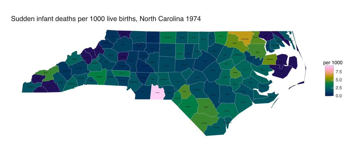
All 100 counties, each named inside its own polygon. Anson, the pink one, recorded 9.55 deaths per 1000 births against a state median of 1.86, and thirteen counties recorded none at all. The band of high rates along the north-eastern border is the kind of pattern a reader can only act on once the counties have names.
Labelling some of them
At 100 labels the type has to be small. Pass a subset as the layer’s own data and only those features get named, at a size that can be read across a room:
top <- nc[order(-nc$rate), ][1:8, ]

p2 <- vplot(nc, width = 10, height = 4.4) |>
  mark_sf(fill = rate, color = "white", linewidth = 0.2) |>
  mark_sf_label(label = NAME, size = 4.2, data = top) |>
  coord_sf() |>
  theme_void() |>
  labs(title = "The eight highest rates", fill = "per 1000")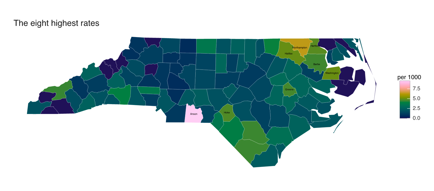
Six of the eight are neighbours in the north-east. The other two, Hoke and Anson, sit on the southern border, which is easier to notice at this size than at 2.6 points.
Why the interior point
The label goes at sf::st_point_on_surface(), which is guaranteed to fall inside the polygon. A centroid is not. Here is a county shaped like a bay:
library(sf)

bay <- st_sf(
  name = "Bay County",
  geometry = st_sfc(st_polygon(list(cbind(c(0, 3, 3, 1, 1, 3, 3, 0, 0),
                                          c(0, 0, 1, 1, 3, 3, 4, 4, 0)))))
)

centre <- st_centroid(st_geometry(bay))
st_within(centre, st_geometry(bay))[[1]]   # empty: the centroid is not in the county
#> integer(0)
mark <- data.frame(st_coordinates(centre), label = "centroid")
p3 <- vplot(bay, width = 5.4, height = 4.2) |>
mark_sf(fill = "#8fb8a8", color = "grey30", linewidth = 0.4) |>
mark_point(x = X, y = Y, data = mark, size = 3, color = "#b5423a") |>
mark_text(x = X, y = Y, label = label, data = mark, size = 4, hjust = 0,
nudge_y = -4, color = "#b5423a") |>
mark_sf_label(label = name, size = 4) |>
theme_void()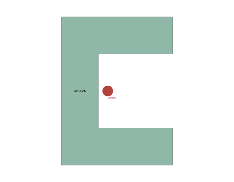
The centroid is in the water. The label is on land. Real coastlines, ring-shaped municipalities and multi-part island counties all have this property, which is why the placement is not a convenience.
Through the projection
The label points are transformed by the same coord_sf() CRS as the geometry, before scale training rather than after, so changing the projection moves the labels with the map instead of stranding them at their unprojected longitude and latitude:
p4 <- vplot(nc, width = 9, height = 4.4) |>
  mark_sf(fill = rate, color = "white", linewidth = 0.2) |>
  mark_sf_label(label = NAME, size = 4.2, data = top) |>
  coord_sf(crs = "EPSG:32119") |>
  theme_void() |>
  labs(title = "The same eight, on the North Carolina state plane",
       fill = "per 1000")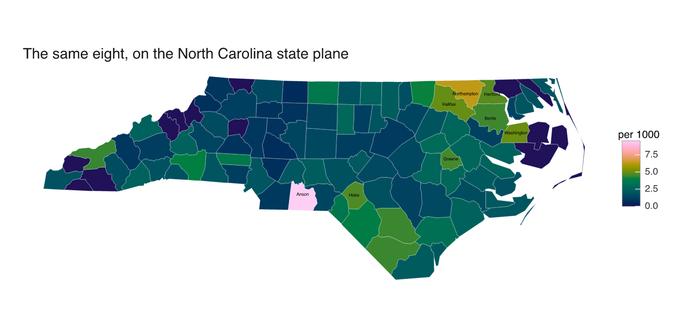
The state is a different shape and every name is still in its county. See Choropleth map for the fill side of this, and Map decorations for scale bars and north arrows.