warm <- linear_gradient(c("#c1121f", "#e08c3a", "#c9a874"))
cool <- linear_gradient(c("#3a5a80", "#6b4f2c"), interpolation = "oklab")

t <- seq(0, 1, length.out = 160)
wave <- function(y, amp, k = 6) y + amp * sin(k * pi * t)

scene <- vl_scene(width = 7, height = 3, dpi = 150, bg = "#faf5ea") |>
  draw(lines_grob(0.04 + 0.92 * t, wave(0.72, 0.12),
                  gp = vl_gpar(col = warm, lwd = 10))) |>
  draw(lines_grob(0.04 + 0.92 * t, wave(0.42, 0.09, k = 4),
                  gp = vl_gpar(col = cool, lwd = 6))) |>
  draw(circle_grob(x = 0.5, y = 0.15, r = 0.1,
gp = vl_gpar(fill = NA, col = warm, lwd = 8)))What a stroke can be
Backend
Gradient strokes, a width and colour per segment, dash phase, an outline you can fill, pixel-snapped hairlines, and haloed text: the paint model applied to lines rather than to fills.
The paint model page is about fills: gradients, patterns, masks, blend modes, all applied to the region a shape encloses. This page is about the region a line covers, which usually gets a colour and a width and nothing else.
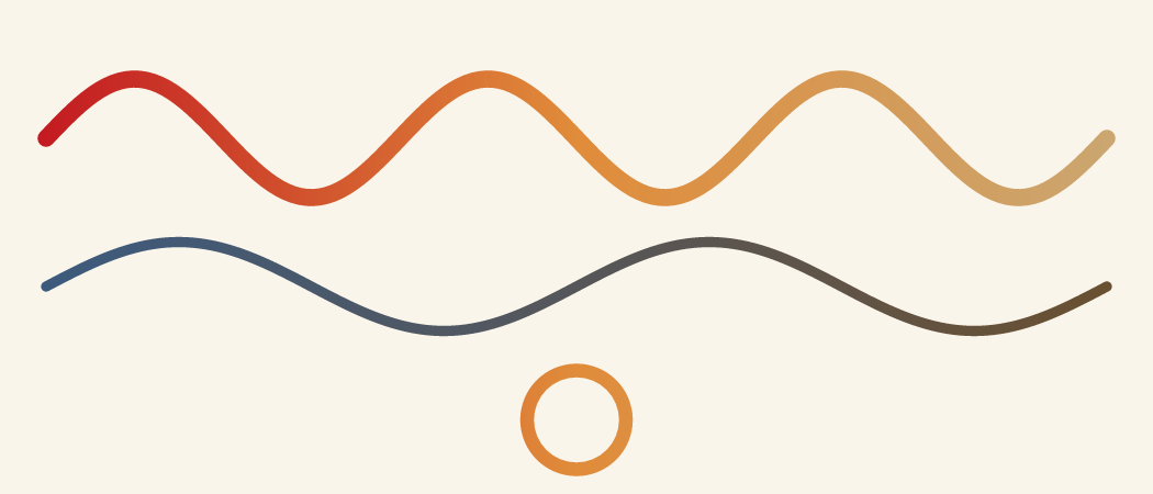
vl_gpar(col = linear_gradient(...)) strokes with a gradient. A trajectory can carry its colour along itself, and it applies to any stroked path: the circle’s outline below is the same paint as the two waves. This is normally faked by emitting a few hundred one-segment lines in slightly different flat colours; here it is one grob and real paint on every backend (a shader in raster, stroke="url(#…)" in SVG, a shading in PDF).
Text and markers fall back to the gradient’s first stop, because a glyph run has no path to run a ramp along. A pattern in col falls back to a flat colour, because a pattern needs cell geometry that a stroke does not have.
A width and a colour per segment
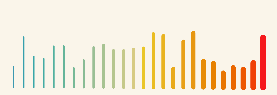
segments_grob() takes a vector of lwd and col, one per segment, in one grob. The saving is not cosmetic: a grob per segment is the R-side cost that dominates busy scenes.
n <- 26
x <- seq(0.05, 0.95, length.out = n)
set.seed(3)
h <- 0.18 + runif(n) * 0.6

bars <- vl_scene(width = 7, height = 2.4, dpi = 150, bg = "#faf5ea") |>
  draw(segments_grob(
    x, 0.08, x, 0.08 + h * 0.8,
    lwd = seq(2, 14, length.out = n),
    col = grDevices::hcl.colors(n, "Zissou1")
  ))
Dash phase
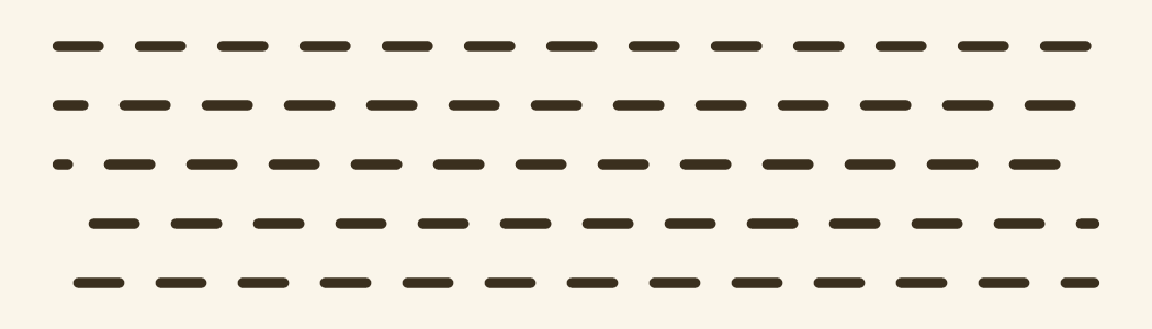
dash_phase sets how far into the dash pattern a line starts, in multiples of lwd, so it scales with the line width exactly as the dashes do. Static, it aligns dashes across adjacent strokes; animated, it is marching ants.
dashes <- vl_scene(width = 7, height = 2, dpi = 150, bg = "#faf5ea")
for (i in 0:4) {
  dashes <- draw(dashes, segments_grob(
    0.05, 0.86 - i * 0.18, 0.95, 0.86 - i * 0.18,
    gp = vl_gpar(col = "#3a2f1e", lwd = 6, lty = "dashed", dash_phase = i * 1.5)
  ))
}
An outline you can fill
stroke_to_path() converts the stroke of a line-like grob into the closed region it covers, the shape you would get by tracing round the drawn line. A one-dimensional path with a colour becomes an area with an interior, so it can be filled with a gradient or a pattern, or handed to a cutting plotter that wants a shape rather than a centreline. It uses the same stroker the rasterizer does, so the outline is exactly the ink that would have landed.
curve <- lines_grob(0.05 + 0.9 * t, 0.5 + 0.3 * sin(3 * pi * t),
                    gp = vl_gpar(lwd = 22))
outline <- stroke_to_path(curve, width = 7, height = 2.4, dpi = 150)

# The outline is a path_grob in millimetres: fill it like any other shape.
filled <- vl_scene(width = 7, height = 2.4, dpi = 150, bg = "#faf5ea") |>
  draw(path_grob(outline@x, outline@y, id = outline@id, rule = "winding",
                 gp = vl_gpar(fill = warm, col = NA)))
The result is baked at one size, and necessarily so: a stroke width is a device quantity, so its outline only exists once a page size and resolution are chosen, and those are arguments here for that reason. An outline is a shape rather than a stroke, so it will not rescale with the page the way the original would.
Hairlines and halos
Two smaller things that decide whether a figure looks sharp or muddy.
vl_gpar(crisp = TRUE) snaps axis-parallel strokes onto the pixel grid. A 1-px rule at a fractional coordinate straddles two rows and renders as two grey ones, and that is why gridlines so often look soft. Snapping puts the rule back on one row; diagonals are left alone. vl_gpar(antialias = FALSE) goes further and gives hard pixel edges, for pixel art, QR codes, and heatmap cells that must tile without a seam.
vl_gpar(halo_col = , halo_width = ) strokes the glyph outlines under the fill, so a label stays legible over a dense scatter or map imagery. Because vellum holds the outlines this is one real stroke rather than the eight offset copies a grid-layered package has to draw, and it works on all three backends. Native SVG uses paint-order, so the text stays selectable.
set.seed(7)
noise <- vl_scene(width = 7, height = 2.4, dpi = 150, bg = "#faf5ea") |>
  draw(points_grob(runif(1200), runif(1200), size = vl_unit(2.6, "mm"),
                   gp = vl_gpar(fill = "#6b4f2c", col = NA, alpha = 0.5))) |>
  draw(text_grob("legible anyway", x = 0.5, y = 0.5,
                 gp = vl_gpar(fontsize = 34, col = "#3a2f1e",
                              halo_col = "#faf5ea", halo_width = 3)))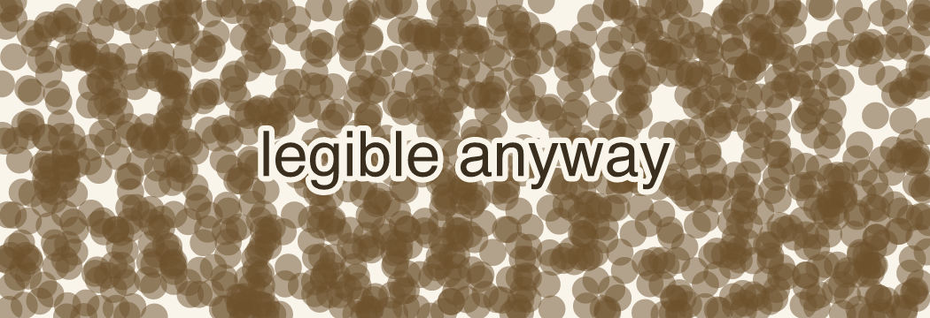
halo_width is in points like fontsize, so the halo keeps its proportion at any dpi.