Contours traced in the engine

mark_contour() and mark_contour_filled() trace iso-lines with vellum’s own marching squares, so contour lines are chained polylines and filled bands are closed rings, with no extra package involved.

A contour plot needs somebody to walk a grid of values and chain the crossings into curves. vellum does that itself (vellum::vl_contour(), marching squares), so mark_contour() needs no tracing package: each contour comes back as one chained polyline, with closed loops actually closed, rather than a heap of disconnected line segments that happen to line up.

The classic two-cluster density: Old Faithful’s eruption lengths against the wait before them.

p <- vplot(faithful, width = 7, height = 4.6) |>
  mark_point(x = eruptions, y = waiting, size = 1.6, color = "#3a2f1e", alpha = 0.5) |>
  mark_contour(x = eruptions, y = waiting, bins = 9, linewidth = 0.7) |>
  labs(
    title = "Old Faithful, contoured",
    x = "eruption length (min)", y = "wait before it (min)", color = "density"
  )

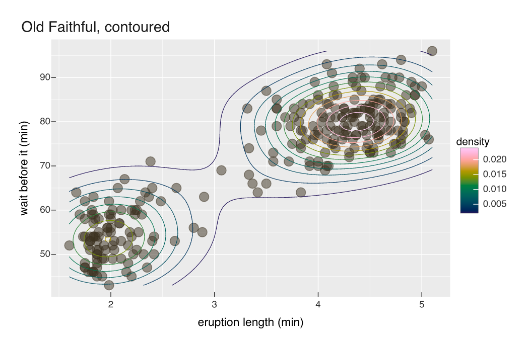
Levels are coloured for you: mark_contour() maps color = after_stat(level), so the legend reads as density without you asking for it.

Filled bands

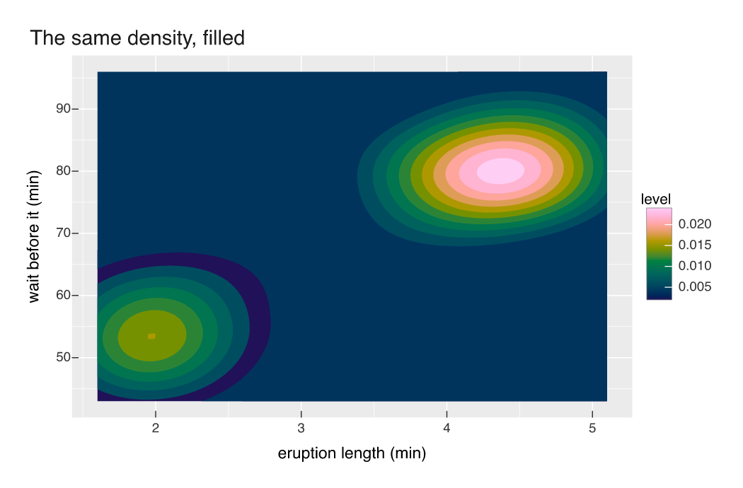
mark_contour_filled() paints the bands between the levels instead. Each band is a closed ring, painted in level order, and that ordering is what produces the layered look. Because the rings are real paths rather than a rasterised heatmap, they stay crisp in SVG and PDF.

A band whose contour runs off the edge of the estimation grid is closed along the grid boundary rather than chorded shut, so the outermost level fills the corners it should instead of slicing wedges across the panel.

p2 <- vplot(faithful, width = 7, height = 4.6) |>
  mark_contour_filled(x = eruptions, y = waiting, bins = 9) |>
  labs(
    title = "The same density, filled",
    x = "eruption length (min)", y = "wait before it (min)", fill = "level"
  )

Contouring a surface you supply

By default the field is a kernel density estimate of the x/y cloud (the one part that still needs MASS). Map a z aesthetic instead and the mark contours your surface over a regular grid: a fitted response, a simulated field, anything you can write as a function of two variables.

grid <- expand.grid(x = seq(-3, 3, length.out = 80), y = seq(-3, 3, length.out = 80))
grid$z <- with(grid, sin(x * 1.4) * cos(y * 1.4) + 0.25 * (x - y))

p3 <- vplot(grid, width = 7, height = 4.6) |>
  mark_contour(x = x, y = y, z = z, bins = 14, linewidth = 0.6) |>
  labs(title = "A supplied surface, not a density", x = NULL, y = NULL, color = "z")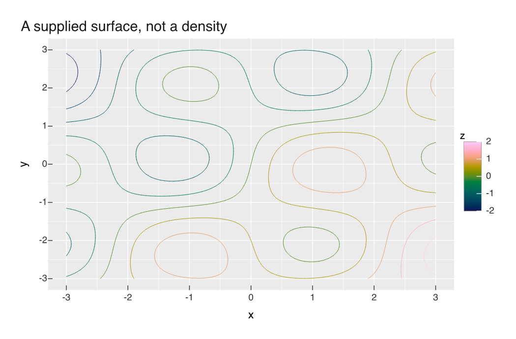

Note the grid convention: like image(), contour(), and outer(), rows index x and columns index y. Pair the lines with mark_text_path() to label a level directly on its own curve instead of through a legend.