vellum is a low-level graphics framework for R, in the spirit of grid. You describe a scene with a small declarative API and render it to PNG, SVG, or PDF.
The property most of the rest follows from is that vellum measures
text and solves layout itself, in process, instead of asking whichever
device happens to be current. So a scene has a size before there is a
page, layout is solved once rather than once per output format, and —
the part with no counterpart in grid — a finished scene can report where
it put every element (scene_model()) and answer what lies
under a given point (hit_test()). That read-back is what an
interactive host, an accessibility layer, or a test suite binds to.
It is the foundation layer a grammar of graphics builds on, the way grid underlies ggplot2. It is not a plotting package itself, so there are no scales, stats, geoms, or facets here. What it gives you is the drawing substrate: units, viewports, grobs, layout, a deterministic renderer, and a scene you can query afterwards.
A first scene
A scene starts with vl_scene(), which fixes the page
size (in inches by default) and background. You then add content with a
pipeline of draw() calls and show the result. Auto-printing
a scene displays it, so the last line of a chunk is enough.
vl_scene(width = 6, height = 3, bg = "white") |>
  draw(rect_grob(
    width = 0.94, height = 0.82,
    gp = vl_gpar(fill = linear_gradient(c("#1b2a4a", "#3a7bd5")), col = NA)
  )) |>
  draw(circle_grob(
    x = 0.16, y = 0.5, r = 0.28,
    gp = vl_gpar(fill = "#f7c948", col = NA)
  )) |>
  draw(text_grob(
    "vellum", x = 0.62, y = 0.5,
    gp = vl_gpar(fontsize = 48, col = "white", fontface = "bold")
  ))
Three ideas do most of the work here.
Grobs are the drawable primitives:
rect_grob(), circle_grob(),
text_grob(), and a couple of dozen more (see
?grob). Each is an immutable value object; building one
draws nothing on its own.
vl_gpar() carries the graphical
parameters (fill, stroke colour, line width, font, opacity) attached to
a grob. A fill can be a plain colour or a gradient, as
above.
Coordinates default to "npc":
normalised parent coordinates, where (0, 0) is the
bottom-left of the region and (1, 1) the top-right. So
x = 0.16 sits near the left edge and y = 0.5
is vertically centred.
Building a scene: push, draw, pop
A scene is a tree of viewports and grobs, built functionally.
push() descends into a new vl_viewport(),
draw() adds a grob at the current level, and
pop() ascends. A viewport is a rectangular region that
establishes its own coordinate systems, so once you push one with an
xscale and yscale, "native" units
map data values straight onto the region.
set.seed(1)
x <- runif(60, 0, 10)
y <- 1.8 * x + rnorm(60, 0, 4)

vl_scene(5, 3.2, bg = "white") |>
  push(vl_viewport(
    x = 0.57, y = 0.57, width = 0.82, height = 0.82,
    xscale = c(0, 10), yscale = range(pretty(y))
  )) |>
  draw(rect_grob(gp = vl_gpar(fill = "#f4f6f8", col = "#cfd8dc"))) |>
  draw(points_grob(
    vl_unit(x, "native"), vl_unit(y, "native"),
    size = vl_unit(3.2, "mm"),
    gp = vl_gpar(fill = "#3a7bd5", col = "#1b2a4a", lwd = 1)
  )) |>
  pop()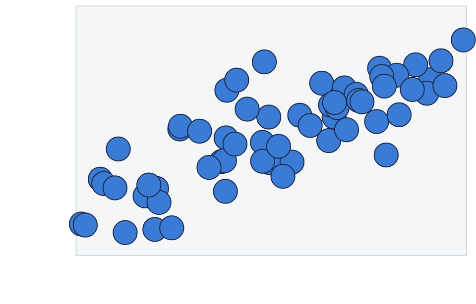
The panel rectangle is drawn in "npc" (it fills its
viewport), while the points are placed in "native" units,
so their positions follow the data scales. A single
vl_unit() vector can even mix coordinate systems per axis.
See vignette("scene-and-paint") for the full picture of
units, viewports, and the paint model.
Rendering to a file
Displaying a scene is convenient while exploring. To write output,
call render(); it picks the backend from the file
extension.
s <- vl_scene(4, 3) |>
  draw(circle_grob(r = 0.3, gp = vl_gpar(fill = "tomato", col = NA)))

render(s, "out.png") # raster (tiny-skia)
render(s, "out.svg") # vector (hand-rolled SVG)
render(s, "out.pdf") # vector (krilla)
The same scene value renders to all three formats with consistent geometry, and raster and PDF output is byte-stable, so it is reproducible and snapshot-testable.
render() takes two arguments worth knowing about.
scale renders at a multiple of the device pixels while
keeping the same physical size — the retina idiom — so nothing about the
layout or the relative size of text changes. cvd simulates
a colour-vision deficiency, which is covered in
vignette("render-quality").
render(s, "out@2x.png", scale = 2) # twice the pixels, same physical size
render(s, "check.png", cvd = "deuteranopia") # as a red/green-blind reader sees it
You do not have to go through a file. Every format is also available in memory, which is what a web handler or an HTML widget wants:
scene_png(s) # raw vector: the encoded PNG
scene_pdf(s) # raw vector: the encoded PDF
scene_svg(s) # character: the SVG document
scene_raster(s) # integer array: the pixels themselves
Where to go next
-
vignette("scene-and-paint"): the scene graph, units and viewports, and the paint model (gradients, patterns, masks). -
vignette("retained-mode"): read back per-element geometry withscene_model(), pick a node under a point withhit_test(), and edit nodes by name. -
vignette("inspecting-scenes"):vl_lint()to catch likely mistakes,scene_stats()for coverage and crowding,profile_render()for where the time goes. -
vignette("render-quality"): colour-vision simulation, crisp gridlines, and group blur/shadow effects. -
vignette("typography"): text halos and OpenType features. -
vignette("coming-from-grid"): a translation guide if you already know grid. -
vignette("grid-interop"): render existing grid, ggplot2, and lattice output through the vellum backend. ```