Every point of interest in Switzerland
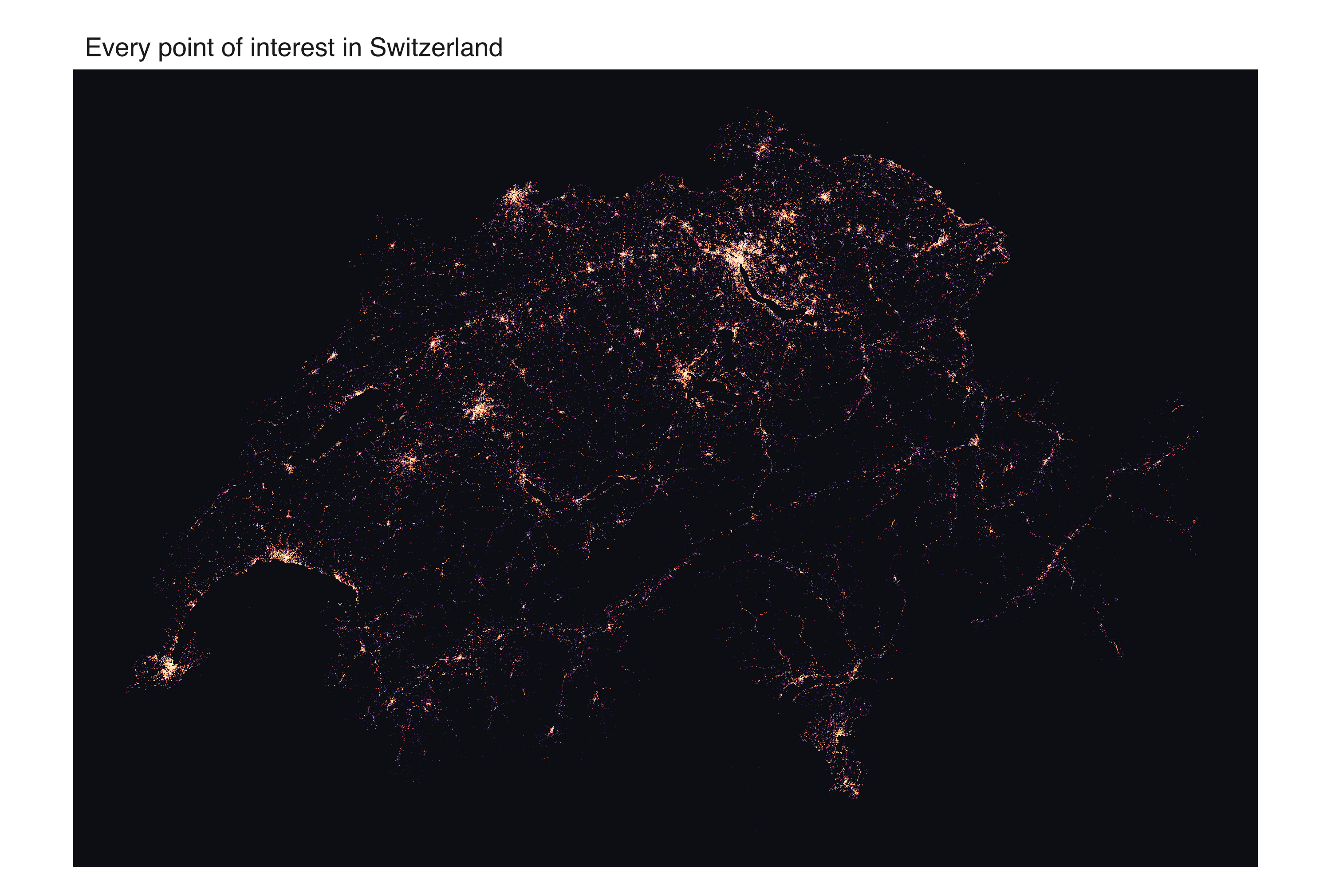
No basemap, no border, no coastline file. Every bright pixel here is a tagged point in OpenStreetMap: a restaurant, a bus stop, a bench, a viewpoint. Plot half a million of them and Switzerland draws itself: the cities glow, the lakes punch dark holes, and the Alpine valleys thin out to single threads of road.
This example is not run when the site is built. It reads a ~500 MB .osm.pbf extract from disk and needs the duckdb, DBI, and arrow packages. The images below are the real output, rendered once and committed with the site; the script at the bottom is the exact source. Grab the input from Geofabrik (switzerland-latest.osm.pbf).
Reading the POIs
The raw PBF holds tens of millions of nodes, ways, and relations. We never load that into R. DuckDB’s spatial extension has ST_ReadOSM(), which streams the file element by element, so the filtering and the Web Mercator projection both happen in SQL. R only ever sees the ~528,000 rows that survive. On a laptop the whole extraction takes a couple of seconds.
A point of interest, for this map, is any node carrying an amenity, shop, tourism, leisure, or public_transport tag. Each one is bucketed into a category from those tags in the same pass.
The map
mark_datashade() aggregates the points into a pixel grid and shades each cell by density. how = "eq_hist" (histogram equalisation) spreads the enormous dynamic range (a bench-lined city block versus an empty pass) across the whole colour ramp, so both stay legible instead of the cities blowing out to white.
One geography per category
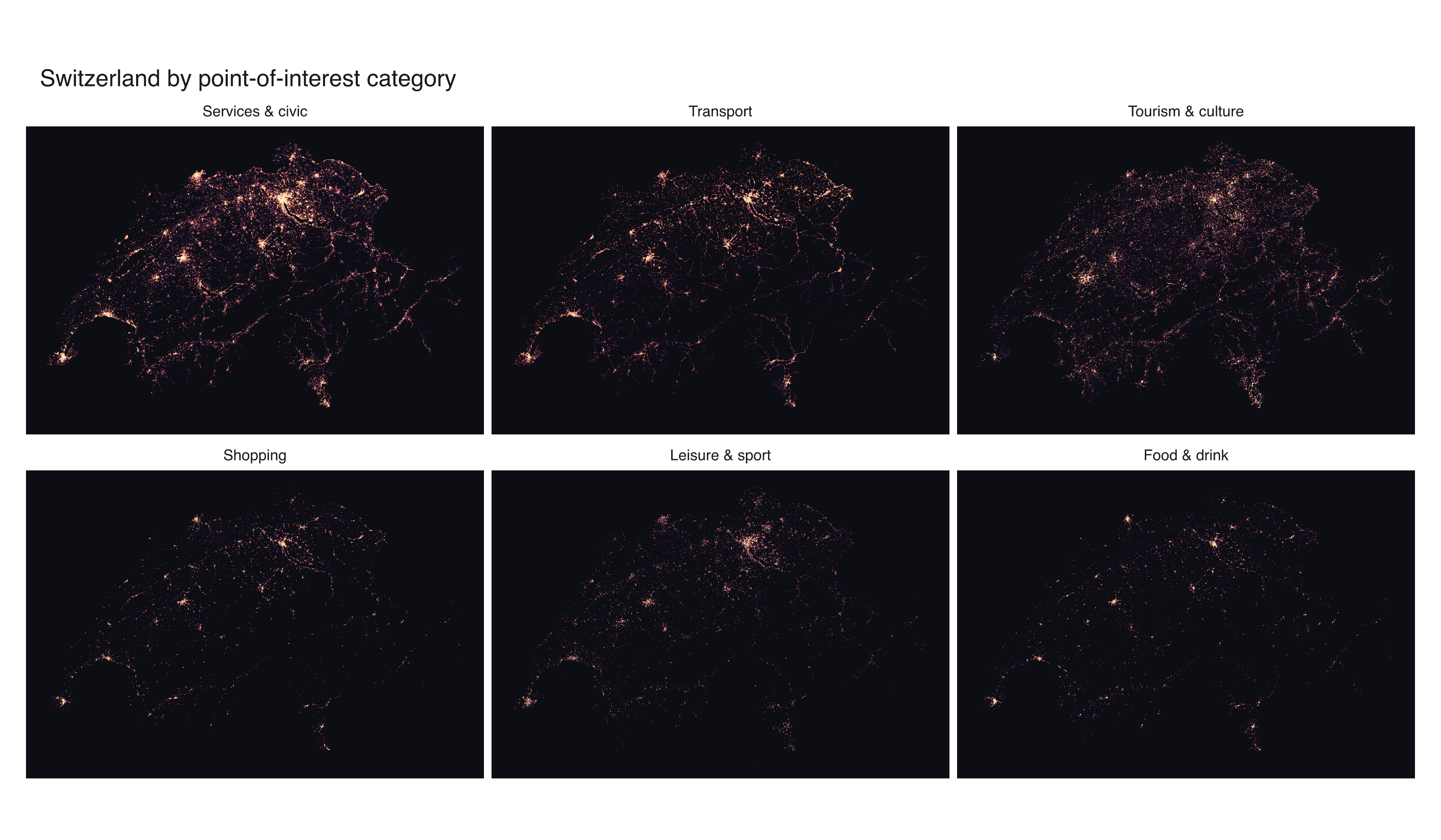
Split the same data by category with facet_wrap() and each POI type turns out to live somewhere different. Transport follows the rail and road network as thin connected lines. Tourism scatters up into the Alps where the viewpoints and huts are. Shopping, food, and leisure collapse back onto the big cities. Services and civic furniture (benches, bins, post boxes) is the densest and the most evenly spread, which is why it traces the country most completely.
The script
# Every point of interest in Switzerland, from an OpenStreetMap extract.
#
# Streams a ~500 MB .osm.pbf with DuckDB's spatial extension, keeps only tagged
# POI nodes, projects them to Web Mercator in SQL, and datashades the ~528k
# survivors with vellumplot -- once as a density map, once faceted by category.
#
# REQUIREMENTS (none are vellumplot dependencies -- this is a heavy showcase):
#   * packages `duckdb`, `DBI`, `arrow`
#   * a Switzerland .osm.pbf, e.g. from
#     https://download.geofabrik.de/europe/switzerland.html

library(DBI)
library(duckdb)
library(arrow)
library(vellumplot)

pbf <- path.expand("~/Downloads/switzerland-latest.osm.pbf")  # <- your file
outdir <- "figures"
dir.create(outdir, showWarnings = FALSE)

# --- 1. Extract POIs with DuckDB -------------------------------------------
# ST_ReadOSM() streams the PBF; all the filtering, categorising, and the
# Web Mercator projection happen in SQL so R only sees the surviving rows.
con <- dbConnect(duckdb())
dbExecute(con, "INSTALL spatial; LOAD spatial;")
dbExecute(con, "SET threads TO 4;")

category_case <- "
  CASE
    WHEN tags['amenity'] IN ('restaurant','cafe','bar','pub','fast_food',
         'biergarten','food_court','ice_cream') THEN 'Food & drink'
    WHEN tags['shop'] IS NOT NULL THEN 'Shopping'
    WHEN tags['tourism'] IS NOT NULL
         OR tags['amenity'] IN ('theatre','cinema','arts_centre','nightclub')
         THEN 'Tourism & culture'
    WHEN tags['public_transport'] IS NOT NULL
         OR tags['amenity'] IN ('parking','bicycle_parking','fuel',
         'charging_station','bicycle_rental','car_sharing','taxi',
         'bus_station','parking_entrance') THEN 'Transport'
    WHEN tags['leisure'] IS NOT NULL
         OR tags['amenity'] = 'fitness_centre' THEN 'Leisure & sport'
    ELSE 'Services & civic'
  END"

query <- sprintf("
  SELECT
    lon * 20037508.34 / 180.0 AS x,                              -- Web Mercator
    ln(tan((90.0 + lat) * pi() / 360.0)) / (pi() / 180.0)
      * 20037508.34 / 180.0 AS y,
    %s AS category
  FROM ST_ReadOSM('%s')
  WHERE kind = 'node'
    AND (tags['amenity'] IS NOT NULL OR tags['shop'] IS NOT NULL
         OR tags['tourism'] IS NOT NULL OR tags['leisure'] IS NOT NULL
         OR tags['public_transport'] IS NOT NULL)
    AND lat IS NOT NULL AND lon IS NOT NULL
", category_case, pbf)

poi <- dbGetQuery(con, query)
dbDisconnect(con, shutdown = TRUE)
message("Loaded ", format(nrow(poi), big.mark = ","), " POIs")

# --- 2. Shared setup -------------------------------------------------------
xr <- range(poi$x); yr <- range(poi$y)
asp <- diff(yr) / diff(xr)                    # equal-aspect (already projected)
ramp <- c("#0d0d14", "#3b1f5e", "#b0246a", "#ff8c42", "#fff2cc")
levels_by_count <- c("Services & civic", "Transport", "Tourism & culture",
                     "Shopping", "Leisure & sport", "Food & drink")
poi$category <- factor(poi$category, levels = levels_by_count)

# --- 3. Density map --------------------------------------------------------
# gw is the datashade grid resolution -- it, not dpi, sets how much detail the
# map holds. Size the page (width * dpi) so the panel is at least gw wide and
# the raster draws close to 1:1 instead of upscaling.
gw <- 2800L
gh <- as.integer(gw * asp)
vplot(poi, width = 10, height = 10 * asp, dpi = 300) |>
  mark_datashade(x = x, y = y, width = gw, height = gh,
                 colors = ramp, how = "eq_hist") |>
  coord_fixed() |>
  theme_void() |>
  set_theme(panel_bg = "#0d0d14") |>
  labs(title = "Every point of interest in Switzerland") |>
  render_plot(file.path(outdir, "swiss-poi-density.png"))

# --- 4. Faceted by category ------------------------------------------------
fgw <- 1200L
fgh <- as.integer(fgw * asp)
vplot(poi, width = 12, height = 7, dpi = 300) |>
  mark_datashade(x = x, y = y, width = fgw, height = fgh,
                 colors = ramp, how = "eq_hist") |>
  facet_wrap(~category) |>
  coord_fixed() |>
  theme_void() |>
  set_theme(panel_bg = "#0d0d14") |>
  labs(title = "Switzerland by point-of-interest category") |>
  render_plot(file.path(outdir, "swiss-poi-category.png"))

message("Wrote 2 figures to ", outdir)