632 million map points, one continent
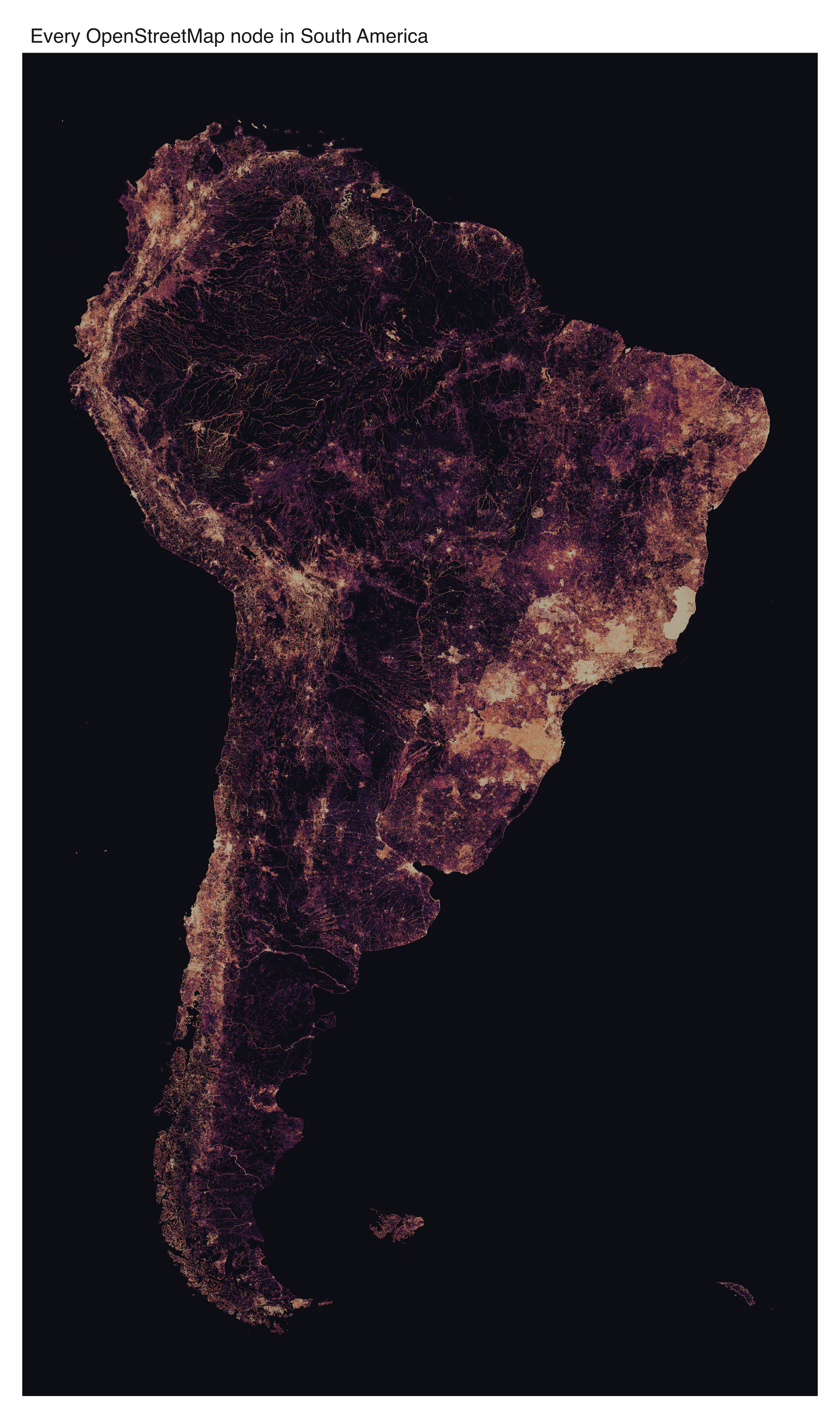
This is every node in the South America OpenStreetMap extract, all 632 million, down to the untagged vertices behind roads, rivers, power lines and building outlines. Drawing all of them traces the continent’s geometry: the braided rivers of the Amazon, the São Paulo–Rio corridor bright along the east coast, the Chilean coast running thin down to Tierra del Fuego.
This example is not run when the site is built. It reads a multi-GB .osm.pbf from disk and needs the duckdb and DBI packages. The image below is the real output, committed with the site; the script at the bottom is the exact source. Grab the input from Geofabrik.
The downsample trick
Handing 632 million points to an in-memory plotting pipeline means holding them in memory first. mark_datashade() aggregates inside R, so every node has to land in an R data frame before anything is drawn, and 632M rows plus the copy R makes to slice them need far more RAM than the machine this ran on had. R stops with a vector memory limit reached error. That ceiling is the hardware, not vellumplot: on a machine with enough memory the same call would draw all 632M directly.
You can sidestep it by looking at what datashading is: a 2D histogram, then a density-to-colour map. Any two points that fall in the same output pixel are identical in the finished image, so there is no reason to move 632 million rows into R when the picture is a few thousand pixels wide. Do the histogram in DuckDB instead: snap each node to a cell of the output grid, GROUP BY the cell, COUNT. Only the non-empty cells come back.
| count | |
|---|---|
| nodes streamed from the PBF | 632,393,976 |
| non-empty cells returned to R | 8,370,415 |
That is a 76× cut, and it costs nothing in the render. Binning to the output grid is what mark_datashade() does internally anyway; this just moves it upstream, where DuckDB streams the file from disk and spills to disk when it has to. R holds only the 8.4M cells, colours them, and draws them with mark_tile(). The result is the same image the in-memory path would have produced, on a machine that could never have held the points.
The map
The grid is 5000 cells wide. eq_hist (histogram equalisation) stretches the count range across the ramp, so the near-empty interior of the Amazon and the dense coast both stay legible in one frame.
The script
# Every OpenStreetMap node in South America (~632 million points), datashaded.
#
# Streams a multi-GB .osm.pbf with DuckDB's spatial extension, aggregates every
# node into a pixel grid IN DUCKDB, and draws the grid with vellumplot. The
# aggregation is the trick: 632M points collapse to ~8.4M non-empty cells, so R
# never has to hold the raw point cloud.
#
# REQUIREMENTS (none are vellumplot dependencies -- this is a heavy showcase):
#   * packages `duckdb`, `DBI`
#   * a South America .osm.pbf from
#     https://download.geofabrik.de/south-america.html

library(DBI)
library(duckdb)
library(vellumplot)

pbf <- path.expand("~/Downloads/south-america-latest.osm.pbf")
outdir <- "figures"
dir.create(outdir, showWarnings = FALSE)
parquet <- file.path(outdir, "south-america-nodes.parquet")

# Mainland frame (lon/lat). Chile's Easter Island (~109 W) and Ecuador's
# Galapagos (~91 W) sit far out in the Pacific; left in they blow the bounding
# box westward and leave the mainland tiny in a field of black. This drops them.
crop <- list(lon = c(-82, -34), lat = c(-56, 13))
gw <- 5000L # output grid width in cells

# --- 1. Extract every node -> Parquet (once) -------------------------------
# ST_ReadOSM() streams the PBF element by element. We keep every node -- tagged
# or not -- and project to Web Mercator in SQL (lat clamped to the valid band).
if (!file.exists(parquet)) {
  con <- dbConnect(duckdb())
  dbExecute(con, "INSTALL spatial; LOAD spatial;")
  dbExecute(con, "SET threads TO 4; SET memory_limit = '12GB';")
  dbExecute(con, sprintf(
    "
    COPY (
      SELECT
        lon * 20037508.34 / 180.0 AS x,
        ln(tan((90.0 + least(85.05, greatest(-85.05, lat))) * pi() / 360.0))
          / (pi() / 180.0) * 20037508.34 / 180.0 AS y
      FROM ST_ReadOSM('%s')
      WHERE kind = 'node' AND lat IS NOT NULL AND lon IS NOT NULL
    ) TO '%s' (FORMAT parquet, COMPRESSION zstd)
  ",
    pbf, parquet
  ))
  dbDisconnect(con, shutdown = TRUE)
}

# --- 2. The downsample trick: aggregate to the grid IN DUCKDB --------------
# Datashading is a 2D histogram + a density-to-colour map, so we do the
# histogram in SQL: snap each node to a cell of the output grid and COUNT. Only
# the non-empty cells (~8.4M of 632M points) come back to R. The parentheses
# around every %.10g matter -- the bounds are negative here, and "x - -1.5e7"
# would splice into "x --1.5e7" where SQL's "--" begins a comment.
con <- dbConnect(duckdb())
dbExecute(con, "SET threads TO 4; SET memory_limit = '12GB';")

mx <- crop$lon * 20037508.34 / 180
my <- log(tan((90 + crop$lat) * pi / 360)) / (pi / 180) * 20037508.34 / 180
where <- sprintf(
  "WHERE x BETWEEN %.10g AND %.10g AND y BETWEEN %.10g AND %.10g",
  mx[1], mx[2], my[1], my[2]
)

b <- dbGetQuery(con, sprintf(
  "SELECT min(x) x0, max(x) x1, min(y) y0, max(y) y1
   FROM read_parquet('%s') %s",
  parquet, where
))
asp <- (b$y1 - b$y0) / (b$x1 - b$x0) # equal-aspect (already projected)
gh <- as.integer(gw * asp)

grid <- dbGetQuery(con, sprintf(
  "SELECT
     least(%d, greatest(0, floor((x - (%.10g)) / ((%.10g) - (%.10g)) * %d)::INT)) AS cx,
     least(%d, greatest(0, floor((y - (%.10g)) / ((%.10g) - (%.10g)) * %d)::INT)) AS cy,
     count(*) AS n
   FROM read_parquet('%s') %s
   GROUP BY 1, 2",
  gw - 1L, b$x0, b$x1, b$x0, gw,
  gh - 1L, b$y0, b$y1, b$y0, gh, parquet, where
))
dbDisconnect(con, shutdown = TRUE)
message(format(nrow(grid), big.mark = ","), " non-empty cells")

# --- 3. Colour (eq_hist) + draw the grid -----------------------------------
# eq_hist (histogram equalisation, datashader's default) is the rank/CDF of the
# cell counts; it spreads the huge dynamic range across the ramp. We colour each
# cell in R and let mark_tile() draw it; scale_fill_identity() passes the hex
# through untouched.
ramp <- c("#0d0d14", "#3b1f5e", "#b0246a", "#ff8c42", "#fff2cc")
eq <- rank(grid$n, ties.method = "average") / nrow(grid)
grid$fill <- grDevices::rgb(grDevices::colorRamp(ramp)(eq), maxColorValue = 255)

vplot(grid, width = 14 / asp, height = 14, dpi = 300) |>
  mark_tile(x = cx, y = cy, fill = fill) |>
  scale_fill_identity() |>
  coord_fixed() |>
  theme_void() |>
  set_theme(panel_bg = ramp[1]) |>
  labs(title = "Every OpenStreetMap node in South America") |>
  render_plot(file.path(outdir, "south-america-nodes-density.png"))