g <- edgebundle::cali2010
xy <- cbind(state.center$x, state.center$y)[
  !state.name %in% c("Alaska", "Hawaii"),
]

p <- vgraph(g, layout = xy) |>
  mark_flow_map(root = "California", weight = weight, width_range = c(0.3, 4)) |>
  mark_nodes(size = 1, fill = "grey30") |>
labs(title = "Migration into California, 2010")Flow map
Networks
A one-to-many flow map: migration into California fans out along merging branches sized by volume.
A flow map shows one source reaching many destinations, the branches merging into trunks whose width grows with the combined flow – the idiom Minard used for Napoleon’s march and cartographers use for migration. mark_flow_map() takes a one-to-many (star) graph laid out at fixed coordinates, the name of the root, and a per-edge weight; the geometry comes from the edgebundle package.
edgebundle::cali2010 records migration into California from every other state in 2010. Placing each state at its geographic centre and rooting the flow at California draws the streams converging on the west coast, each trunk sized by how many people moved along it.
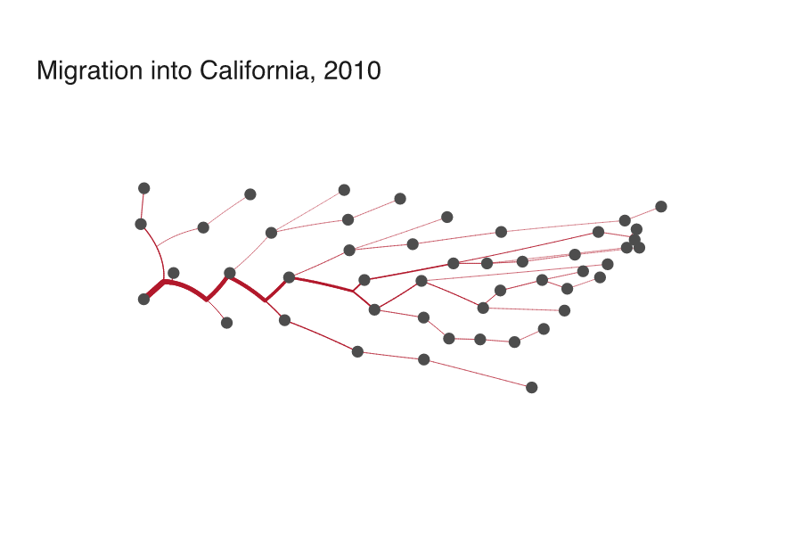
type = "spiral" (the default) is an angle-restricted spiral tree: planar, crossing-free, and needing only the edgebundle package. type = "steiner" builds an approximate Steiner tree instead (it additionally needs the interp package). The computed flow is mapped onto width_range, so the busiest trunk stays legible however lopsided the volumes are.