peng <- na.omit(datasets::penguins)
spec_fields(peng)
#>          name         type   class n_unique                        examples
#> 1     species      nominal  factor        3 Adelie   , Gentoo   , Chinstrap
#> 2      island      nominal  factor        3 Torgersen, Biscoe   , Dream
#> 3    bill_len quantitative numeric      163                39.1, 39.5, 40.3
#> 4    bill_dep quantitative numeric       79                18.7, 17.4, 18.0
#> 5 flipper_len quantitative integer       54                   181, 186, 195
#> 6   body_mass quantitative integer       93                3750, 3800, 3250
#> 7         sex      nominal  factor        2                  male  , female
#> 8 year quantitative integer 3 2007, 2008, 2009A chart an agent writes as data, not as code
Backend
spec_fields() grounds a model in the real columns, vplot_from_spec() validates what it produces and reports the mistake as a record, mcp_serve() exposes both to an MCP client, and provenance_join() says which rows drew each element.
Ask a language model for a plot and you normally get R code, which you then have to run. Executing generated code is the part nobody wants to defend, and the failure mode is bad: the model invents a column name, the script throws, and you get a traceback written for a human debugging their own typo.
Because a vellumplot plot is a spec, the model can produce the document instead. Nothing is executed. Three functions cover the loop: one to tell the model what the data actually contains, one to check what came back, and one to serve both over the Model Context Protocol.
Telling the model what the columns are
spec_fields() is the grounding step. One row per column, with the encoding type a spec would use, how many distinct values it has, and a few real ones:
Hallucinated field names mostly come from the model guessing at a schema it was never shown. Hand it this table first and the guessing stops.
Compiling what it wrote
A spec is JSON, so this is the whole payload for a coloured scatter:
spec <- '{
  "version": "1",
  "width": 6.5, "height": 4, "dpi": 150,
  "data": {"name": "penguins"},
  "layers": [
    {"mark": "point",
     "encoding": {
       "x": {"field": "flipper_len", "type": "quantitative"},
       "y": {"field": "body_mass", "type": "quantitative"},
       "color": {"field": "species", "type": "nominal"}}}
  ],
  "labels": {"title": "Flipper length against body mass",
             "x": "flipper length (mm)", "y": "body mass (g)",
             "color": "species"}
}'

p <- vplot_from_spec(spec, data = peng)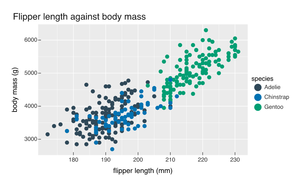
vplot_from_spec() validates every referenced field against the data and dry-runs the compile before handing back a PlotSpec. Get a name wrong and the error is a record rather than a stack trace: which field, what was expected, what exists.
vplot_from_spec(sub("flipper_len", "flipper_length", spec, fixed = TRUE), data = peng)
#> Error in `vplot_from_spec()`:
#> ! Invalid spec:
#> ✖ Unknown field 'flipper_length'. Available fields: species, island, bill_len,
#>   bill_dep, flipper_len, body_mass, sex, year.
spec_diagnose() is the same check without the throw, for a caller that would rather branch on $ok and retry.
Over MCP
mcp_serve() puts that behind three tools: get_schema, list_fields, and render_spec. It speaks newline-delimited JSON-RPC 2.0 on stdio, in pure R, so registering it takes one line:
claude mcp add vellumplot -- Rscript -e 'vellumplot::mcp_serve()'Nothing about it is specific to a client, and the protocol is plain enough to speak by hand. Start one server, hand it a handshake and three tool calls on stdin, and read the replies back off stdout:
csv <- file.path(tempdir(), "penguins.csv")
write.csv(peng, csv, row.names = FALSE)

req <- function(id, method, params = list()) {
  jsonlite::toJSON(list(jsonrpc = "2.0", id = id, method = method, params = params),
                   auto_unbox = TRUE)
}
call <- function(id, name, arguments) {
  req(id, "tools/call", list(name = name, arguments = arguments))
}

session <- c(
  req(1, "initialize"),
  req(2, "tools/list"),
  call(3, "list_fields", list(data_path = csv)),
  call(4, "render_spec", list(spec = spec, data_path = csv,
                              out_path = "figs/agent-specs-mcp.png")),
  call(5, "render_spec", list(spec = sub("body_mass", "mass", spec, fixed = TRUE),
                              data_path = csv))
)

out <- system2("Rscript", c("-e", shQuote("vellumplot::mcp_serve()")),
               input = session, stdout = TRUE)
replies <- lapply(out, jsonlite::fromJSON, simplifyVector = FALSE)

length(replies)
#> [1] 5
replies[[1]]$result$serverInfo
#> $name
#> [1] "vellumplot"
#>
#> $version
#> [1] "0.9.0.9000"
vapply(replies[[2]]$result$tools, `[[`, character(1), "name")
#> [1] "get_schema"  "list_fields" "render_spec"
Five requests, five replies, one process. Request 3 is list_fields, which hands back the same table spec_fields() printed above, this time as JSON. Request 4 renders, and reports where it put the file:
cat(replies[[4]]$result$content[[1]]$text)
#> {
#>   "ok": true,
#>   "path": "figs/agent-specs-mcp.png"
#> }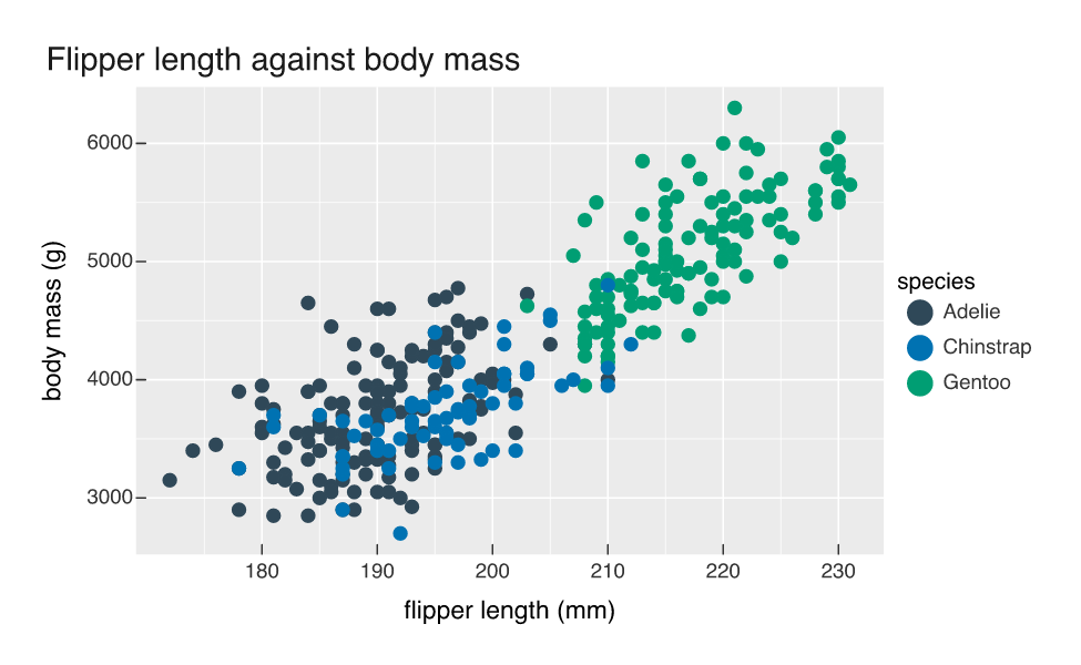
That figure came out of the server, not out of this page. The agent never saw R code and the host never ran any. The fifth request is the same spec with one field renamed, and it comes back the same shape as the error above, flagged as a tool error so the client knows to repair rather than report:
replies[[5]]$result$isError
#> [1] TRUE
cat(replies[[5]]$result$content[[1]]$text)
#> {
#>   "ok": false,
#>   "diagnostics": [
#>     {
#>       "severity": "error",
#>       "field": "mass",
#>       "message": "Unknown field 'mass'.",
#>       "hint": "Available fields: species, island, bill_len, bill_dep, flipper_len, body_mass, sex, year."
#>     }
#>   ]
#> }
That hint is what turns a retry into a fix instead of another guess.
Which rows drew this element
The other half of an agent’s problem is reading a figure back. provenance_join() compiles the plot once and returns one row per drawn element, carrying both the source rows that produced it and where it landed in device pixels:
pj <- provenance_join(p)
pj[, c("id", "layer", "mark", "x", "y", "w", "h", "n_rows")]
#>                 id layer  mark        x       y        w        h n_rows
#> 1 layer-1-point-g1     1 point 341.3842 373.972 406.9720 217.0845    146
#> 2 layer-1-point-g2     1 point 623.5349 226.146 302.9823 262.4046    119
#> 3 layer-1-point-g3     1 point 400.8746 371.101 365.3761 235.7457     68
The scatter draws as three grobs, one per species, so each row here covers a whole group and its bounding box. rows is a list column of indices back into the data:
head(peng[pj$rows[[3]], c("species", "flipper_len", "body_mass")], 4)
#>       species flipper_len body_mass
#> 277 Chinstrap         192      3500
#> 278 Chinstrap         196      3900
#> 279 Chinstrap         193      3650
#> 280 Chinstrap         188      3525
Given a pixel, the boxes say which element was hit and the indices say what it means, which is the substrate under linked views and click-to-source. It is also how a figure gets audited, since every element can name the data behind it. The hashing side of the same idea is in A figure that carries its own provenance.